4. Xgboost

XGBoost initially started as a research project by Tianqi Chen as part of the Distributed (Deep) Machine Learning Community (DMLC) group. Initially, it began as a terminal application which could be configured using a libsvm configuration file. It became well known in the ML competition circles after its use in the winning solution of the Higgs Machine Learning Challenge. Soon after, the Python and R packages were built, and XGBoost now has package implementations for Java, Scala, Julia, Perl, and other languages. This brought the library to more developers and contributed to its popularity among the Kaggle community, where it has been used for a large number of competitions.

It was soon integrated with a number of other packages making it easier to use in their respective communities. It has now been integrated with scikit-learn for Python users and with the caret package for R users. It can also be integrated into Data Flow frameworks like Apache Spark, Apache Hadoop, and Apache Flink using the abstracted Rabit and XGBoost4J. XGBoost is also available on OpenCL for FPGAs. An efficient, scalable implementation of XGBoost has been published by Tianqi Chen and Carlos Guestrin.

While the XGBoost model often achieves higher accuracy than a single decision tree, it sacrifices the intrinsic interpretability of decision trees. For example, following the path that a decision tree takes to make its decision is trivial and self-explained, but following the paths of hundreds or thousands of trees is much harder. To achieve both performance and interpretability, some model compression techniques allow transforming an XGBoost into a single “born-again” decision tree that approximates the same decision function.

4.1. The algorithm

XGBoost works as Newton-Raphson in function space unlike gradient boosting that works as gradient descent in function space, a second order Taylor approximation is used in the loss function to make the connection to Newton Raphson method.

A generic unregularized XGBoost algorithm is:

Input: training set \(\{(x_{i},y_{i})\}_{i=1}^{N}\), a differentiable loss function \(L(y, F(x))\), a number of weak learners M and a learning rate \(\alpha\).

Algorithm:

1. Initialize model with a constant value:

   \[\hat{f}_0(x) = arg_{\theta}\quad min \sum_{i=1}^N L(y_i,\theta)\]

2. For m = 1 to M:

   2.1 Compute the ‘gradients’ and ‘hessians’:

   \[\begin{split}\begin{aligned} \hat{g}_m(x_i) &= \left[\frac{\partial L(y_i,f(x_i))}{\partial f(x_i)} \right]_{f(x)=\hat{f}_{m-1}(x)}\\ \hat{h}_m(x_i) &= \left[\frac{\partial^2 L(y_i,f(x_i))}{\partial^2 f(x_i)} \right]_{f(x)=\hat{f}_{m-1}(x)}\\ \end{aligned}\end{split}\]

   2.2 Fit a base learner (or weak learner, e.g. tree) using the training set \(\{ x_i, -\frac{\hat{g}_m(x_i)}{\hat{h}_m(x_i)} \}_{i=1}^N\) , by solving the optimization problem below:

   \[\begin{split}\begin{aligned} \hat{\phi}_m &= arg_{\theta}\quad min \sum_{i=1}^N \frac{1}{2}\hat{h}_m(x_i) \left[ \phi(x_i) -\frac{\hat{g}_m(x_i)}{\hat{h}_m(x_i)} \right]^2 \\ \hat{f}_m(x) &= \alpha \hat{\phi}_m(x) \end{aligned}\end{split}\]

   2.3 Update the model:

   \[\hat{f}_{(m)}(x) = \hat{f}_{(m-1)}(x) + \hat{f}_m(x)\]

3. Output:

   \[\hat{f}(x) = \hat{f}_{(M)}(x) = \sum_{m=0}^M \hat{f}_{m}(x)\]

4.2. Build Model

To build the model with mlita package.

from mlita.ml import MachineLearning
import numpy as np

model = MachineLearning.from_csv('./data/nmr_O.csv')
print(model.data.shape)
print(model.x_data.shape)
print(model.y_data.shape)

(209, 13)
(209, 12)
(209,)

# 超参调整
params={'max_depth':8,
    'n_estimators':29,
    'min_child_weight':8,
    'subsample':0.9,
    'colsample_bytree':0.6,
    'reg_alpha':0.1,
    'reg_lambda':0.7
    }
model_xgboost = model.xgboost(params=params)
x_test = np.random.rand(1,12)
model_xgboost.predict(x_test)

array([30.750021], dtype=float32)

4.3. Save Data

model.to_csv()

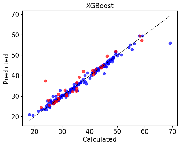
scores = model.make_score()
scores

{'mse': 8.575921681875219,
 'mae': 1.7102975633621214,
 'r2': 0.9003680781166987,
 'r': 0.9543486060650683}

4.4. Plot

model.save_picture()

True